EODataDown – user guidance
Analysis ready data (ARD) - specifications
The EODataDown platform (https://livingwales.aber.ac.uk) provides access to and visualisations of Analysis Ready Data (ARD) satellite data for Wales, namely those acquired by Sentinel-1 (C-band radar) and Sentinel-2 and Landsat (optical). These data have been processed to a minimum set of requirements and organized into a form that allows i) immediate analysis with a minimum of additional user effort and ii) interoperability both through time and with the same and other datasets (https://ceos.org/ard/).
Projection and coordinate system
All data are being provided within the Ordnance Survey of Great Britain (OSGB36) / British National Grid -- United Kingdom Ordnance Survey (EPSG:27700) projection system (https://epsg.io/27700).
Satellite sensor data
Sentinel-2
The ESA-Copernicus Sentinel-2 mission includes two polar-orbiting satellites that each support the optical MultiSpectral Instrument (MSI). These satellites have been placed in the same sun-synchronous orbit and are phased at 180° to each other. Each satellite images a swath of approximately 290 km every 10 days, but as there are two in orbit, the Earth is observed every 5 days at the Equator and as much as 2-3 days at higher latitudes.
The Sentinel-2 multi-spectral data that are provided for Wales have been downloaded from ESA-Copernicus as an atmospherically corrected (Level2-A) product and have a spatial resolution of between 10 - 20 metres (depending on the spectral band). The 60-m resolution spectral bands (i.e., Band 1, 9 and 10) are not provided on the EODataDown platform. All data have been reprojected to the British National Grid (EPSG: 27700). The different spectral bands are listed in Table 1 and a shadow/cloud layer (SCL) is also provided.
Table 1: Sentinel-2 bands and characteristics
| Band No | Wavelength region | Central wavelength (µm) | Resolution (m) |
|---|---|---|---|
| 1 | Coastal aerosol | 0.443 | 60 |
| 2 | Blue | 0.490 | 10 |
| 3 | Green | 0.560 | 10 |
| 4 | Red | 0.665 | 10 |
| 5 | Vegetation red edge | 0.705 | 20 |
| 6 | Vegetation red edge | 0.740 | 20 |
| 7 | Vegetation red edge | 0.783 | 20 |
| 8 | Near infrared | 0.842 | 10 |
| 8A | Vegetation red edge | 0.865 | 20 |
| 9 | Water vapour | 0.945 | 60 |
| 10 | Shortwave infrared (Cirrus) | 1.375 | 60 |
| 11 | Shortwave infrared | 1.610 | 20 |
| 12 | Shortwave infrared | 2.190 | 20 |
All the reflectance products are distributed in separate GeoTiff files with a scaling factor of 10,000 (Table 2).
Table 2: Specifications of distributed Sentinel-2 data
| Period | January 2017 – today * | |
|---|---|---|
| Sensor | Multispectral Instrument (MSI) | |
| Process Level | Level2-A | |
| Distributed CRS | EPSG: 27700 (British National Grid) | |
| Format | Geotiffs (one per band) | |
| Cell Size (metres) | 10: Bands 2-4 and 8 20: Bands 5-7,8A and 11-12 |
|
| Value Ranges | Band 2-12: 1-10000 Shadow/Cloud Layer (SCL): 1-11 |
|
| NoData Value | 0 | |
| SCL Values | 1: saturated or defective 2: dark area pixels 3: cloud shadows 4: vegetation 5: not vegetated 6: water 7: unclassified 8: cloud medium probability 9: cloud high probability 10: thin cirrus 11: snow |
|
| Product Unit | Band 2-12: reflectance, SCL: None |
*Jan-Mar 2017: Processed to L2A from L1C by Living Wales using Sen2Cor 2.5.5 version, Apr-today: official ESA-Copernicus L2A product.
Warning: ESA-Copernicus is only providing Sentinel-2 Level2-A products for the April 2017–present period. To provide data for the full 2017 year, the three missing months (i.e., Jan-Mar) were processed by Living Wales from Level1-C Copernicus products to Level2-A using the official Copernicus Sen2Cor version 2.5.5 software. Whereas, the 2017 (Apr-Dec) ESA-Copernicus Level2-A products were generated using Planet-Digital Elevation Model (DEM) (90 m), Sen2Cor Version 2.5.5 software uses the SRTM-DEM (90 m). Also, additional auxiliary data (e.g., monthly snow conditions) have been used by ESA-Copernicus within Sen2Cor.
A comparison between the atmospherically corrected (Level2-A) reflectance products generated using Sen2Cor Version 2.5.5 and the official ESA-Copernicus products (for scenes acquired in May 2017) has shown the absolute reflectance values differ slightly but the reflectance profiles follow the same patterns (Appendix 1-2).
Sentinel-1
The ESA Sentinel-1 mission was comprised of a constellation of two polar-orbiting satellites supporting a C-band Synthetic Aperture Radar (SAR) that is able to acquire data both day and night and regardless of most atmospheric conditions. This is particularly relevant to Wales, as cloud cover is persistent but nevertheless images are acquired. Each satellite was designed to revisit every 12 days at the Equator and 6 days with the two satellites, but between the latitudes where Wales is positioned, data are acquired every 1-3 days.
Sentinel-1 Level-1 High-Resolution Dual-Polarization (GRD-HD) data acquired with Interferometric Wide swath (IW) mode have been downloaded from the Alaska Satellite Facility (ASF) and processed to an ARD form (i.e., Radiometrically Terrain Corrected (RTC) gamma0 backscatter, in decibel (dB) and with British National Grid (EPSG: 27700) projection) with a 10-metre pixel resolution using ESA's SNAP software (Table 3). Distributed Sentinel-1 data include both VH (Vertically transmitted, Horizontally received) and VV polarizations (in separate GeoTiff files).
Table 3: Specifications of distributed Sentinel-1 data
| Period | Mar 2015 - today | |
|---|---|---|
| Sensor | C-SAR | |
| Acquisition mode | Interferometric Wide swath (IW) | |
| Polarization | VV+VH | |
| Process Level | RTC | |
| Product Type | gamma0 | |
| Product Unit | decibel (dB) | |
| NoData Value | 0 | |
| Distributed CRS | EPSG: 27700 (British National Grid) | |
| Format | Geotiffs (one per band) | |
| Cell Size (metres) | 10 | |
| Parent Dataset | L1 Detected High-Res Dual-Pol (GRD-HD) |
Landsat (not available yet)
The Landsat program offers the longest continuous global record of the Earth’s surface (i.e., since 1988).
Landsat scenes have been downloaded from the United States Geological Survey (USGS) Collection 2 archive as an atmospherically corrected (ARD product (Level-2)) with a 30 metre pixel resolution and all data have been reprojected to British National Grid (EPSG: 27700).
Viewing and downloading satellite data
Filtering (period, sensor, and region of interest)
To visualise and/or download satellite data (i.e., ARD), the first step is to select a period, sensor, and region of interest.
Period of interest
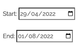
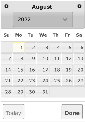
To specify a period of interest, enter the start and end dates using the calendar pop-up (Figure 1). Periods of available data, for each satellite, are specified in Section 1.2 and summarised in Table 2 and Table 3, respectively for Sentinel-2 and Sentinel-1. By default, the period of interest is set to 3 months with the end date being “today”. At any time, you can reset the changes you have made and set the end date to “today” by clicking on the  button in the calendar pop-up (Figure 1b).
|
b)
|
|
|---|---|---|
| Figure 1: Selecting a period of interest, i.e., a) defining a start date and end date, using b) the calendar pop-up. |
Sensor of interest
The next step is to specify a sensor of interest. Select your sensor of choice in the drop-down menu (Figure 2). By default, Sentinel-1 SAR is selected.
Note: Currently, only Sentinel-1 and Sentinel-2 are available. Landsat will be released by the end of the project.
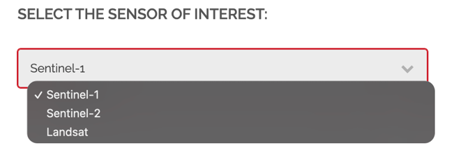
Figure 2: Selecting a sensor of interest
Cloud percentage threshold (optional)
If you have selected an optical sensor (i.e., Sentinel-2 or Landsat) in Section 2.1.2, you can specify a cloud cover (%) maximum threshold. By default, all images are included (i.e., cloud cover (%) set to 100), but the option is there for you to filter these based on cloud cover (%).
Region of interest (optional)
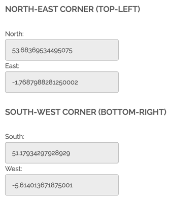
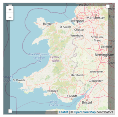
Finally, you can specify a region of interest (i.e., using a bounding box) by either a) directly entering the North, East, South, West coordinates (in degrees - EPSG: 4326) in the boxes (see Figure 3a), or b) using the interactive map (see Figure 3b). When using the interactive map, drag a corner to change the size of the bounding box, and pan and zoom the map to specify the area of interest; the coordinate values are automatically updated.
By default, the region of interest is set to the maximum extent (i.e., the whole Wales, as shown in Figure 3).
a)
|
b)
|
|
|---|---|---|
| Figure 3: Selecting a region of interest by either a) directly entering the coordinate values, or b) interactively using the map. |
Sending request
Once all the specifications have been entered (c.f., Section 2.1.1. - 2.1.4.), please click on the  button to request the scenes. All the available scenes for the indicated sensor, period, and extent (and maximum cloud cover in case of optical sensor) will be listed, with a small pre-view, on this “ImageList” page.
Viewing
To visualise a larger pre-view of a scene or its metadata, from the “ImageList” page (see Section 2.1.5.), you can either click on “Map” or “Quicklook”. The two types of pages provide the same information, with the exception of the pre-view, which is overlayed on top of an interactive background (i.e., Open Street Map or Google Earth image) in the “Map” pages. In the “Quicklook” pages, the pre-view is a standalone layer and therefore is quicker to load. Depending on your internet connection, please select the most convenient option.
Note: Once you are on the “Map” or “Quicklook” page of a scene, you can always go back to the full list of your requested scenes (i.e., “ImageList” page) by clicking on Back to image list at the top of the page.
In the “Map” pages, click on the  button to select the background of your choice (i.e., Open Street Map or Google Earth image), and to view/un-view the scene’s pre-view. You can zoom in and move the map to obtain a more detailed visualisation of an area. By default, the zoom level is set to have a general view of the scene.
Note: the spatial resolution of pre-views has been degraded compared to the original data to give a more streamlined experience with common internet bandwidths. Downloaded data are all with original (i.e., full) resolution.
For each scene, the “Map”/“Quicklook” page contains all the metadata. The full list is available in Table 4.
Table 4: List of metadata with relevant sensors
| Field | Sensor |
|---|---|
| Scene ID | Sentinel-1, Sentinel-2 |
| Sensing Time | Sentinel-1, Sentinel-2 |
| Sensor/Instrument | Sentinel-1, Sentinel-2 |
| Platform | Sentinel-1, Sentinel-2 |
| MGRS Tile | Sentinel-2 |
| Datatake Identifier | Sentinel-2 |
| Absolute Orbit | Sentinel-1 |
| Relative Orbit | Sentinel-1 |
| Doppler | Sentinel-1 |
| Flight Direction | Sentinel-1 |
| Look Direction | Sentinel-1 |
| Acquisition mode | Sentinel-1 |
| Polarization | Sentinel-1 |
| Process Description | Sentinel-1, Sentinel-2 |
| Process Level | Sentinel-1, Sentinel-2 |
| Product Type | Sentinel-1 |
| Product Unit | Sentinel-1, Sentinel-2 |
| Value Range | Sentinel-2 |
| NoData Value | Sentinel-1, Sentinel-2 |
| SCL Value | Sentinel-2 |
| Parent Dataset. | Sentinel-1 |
| Distributed CRS | Sentinel-1, Sentinel-2 |
| Cell Size (metres) | Sentinel-1, Sentinel-2 |
| Cloud Cover (%) | Sentinel-2 |
| North Lat. (degrees) | Sentinel-1, Sentinel-2 |
| South Lat. (degrees) | Sentinel-1, Sentinel-2 |
| East Lon. (degrees) | Sentinel-1, Sentinel-2 |
| West Lon. (degrees) | Sentinel-1, Sentinel-2 |
Downloading
All the ARD scenes are freely downloadable from the EODataDown platform, and more precisely at the bottom of the “Map” and “Quicklook” pages (see Section 2.2). The scene bands/products are distributed in separate download links and are in a GeoTiff format and at full spatial resolution. To download the bands/products, you will need a username and password. Please email livingwales-data@aber.ac.uk to request your account IDs. The username and password will be sent to you via a private email.
Appendix 1: Laugharne - River Tâf - River Towy transect
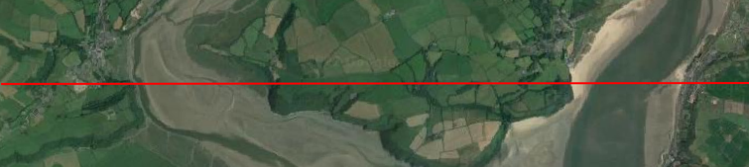
Figure A1-1: Localisation of the Laugharne-River Tâf- River Towy transect
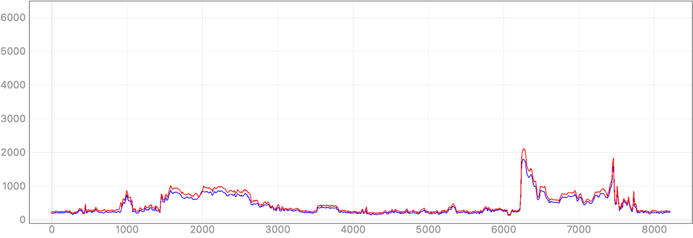
Figure A1-2: Band 2 (i.e., blue band) reflectance (with a scaling factor of 10,000) profiles for the ESA-Copernicus (in blue) and Sen2Cor version 2.5.5 (in red) Level2-A products (on 8 May 2017), Laugharne-River Tâf- River Towy transect.
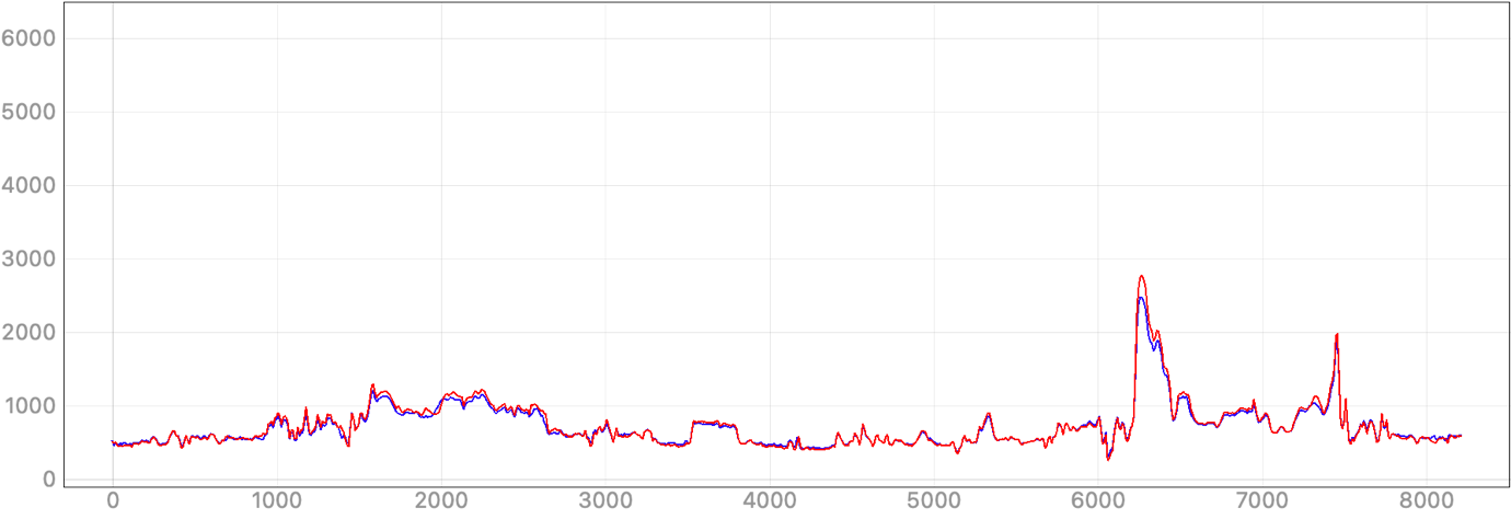
Figure A1-3: Band 3 (i.e., green band) reflectance (with a scaling factor of 10,000) profiles for the ESA-Copernicus (in blue) and Sen2Cor version 2.5.5 (in red) Level2-A products (on 8 May 2017), Laugharne-River Tâf- River Towy transect.
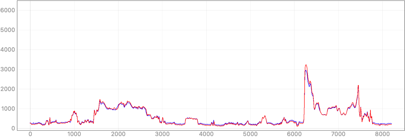
Figure A1-4: Band 4 (i.e., red band) reflectance (with a scaling factor of 10,000) profiles for the ESA-Copernicus (in blue) and Sen2Cor version 2.5.5 (in red) Level2-A products (on 8 May 2017), Laugharne-River Tâf- River Towy transect.
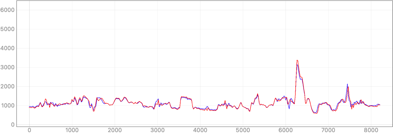
Figure A1-5: Band 5 (i.e., vegetation red edge) reflectance (with a scaling factor of 10,000) profiles for the ESA-Copernicus (in blue) and Sen2Cor version 2.5.5 (in red) Level2-A products (on 8 May 2017), Laugharne-River Tâf- River Towy transect.
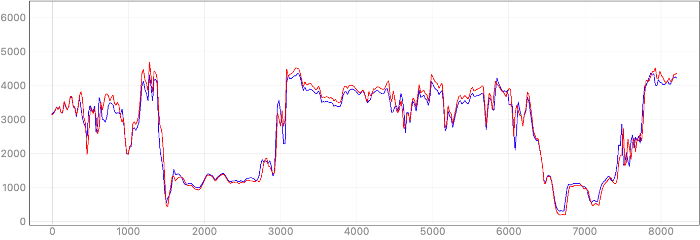
Figure A1-6: Band 6 (i.e., vegetation red edge) reflectance (with a scaling factor of 10,000) profiles for the ESA-Copernicus (in blue) and Sen2Cor version 2.5.5 (in red) Level2-A products (on 8 May 2017), Laugharne-River Tâf- River Towy transect.
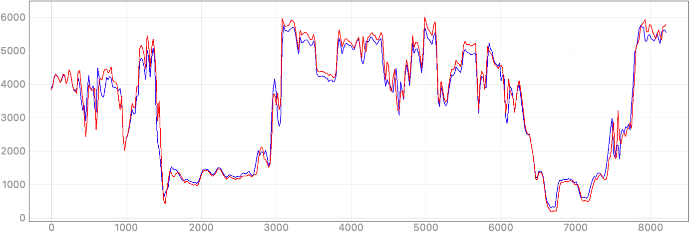
Figure A1-7: Band 7 (i.e., vegetation red edge) reflectance (with a scaling factor of 10,000) profiles for the ESA-Copernicus (in blue) and Sen2Cor version 2.5.5 (in red) Level2-A products (on 8 May 2017), Laugharne-River Tâf- River Towy transect.
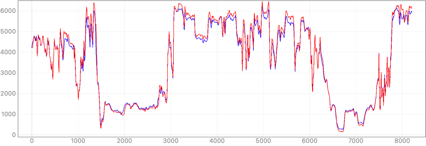
Figure A1-8: Band 8 (i.e., NIR band) reflectance (with a scaling factor of 10,000) profiles for the ESA-Copernicus (in blue) and Sen2Cor version 2.5.5 (in red) Level2-A products (on 8 May 2017), Laugharne-River Tâf- River Towy transect.
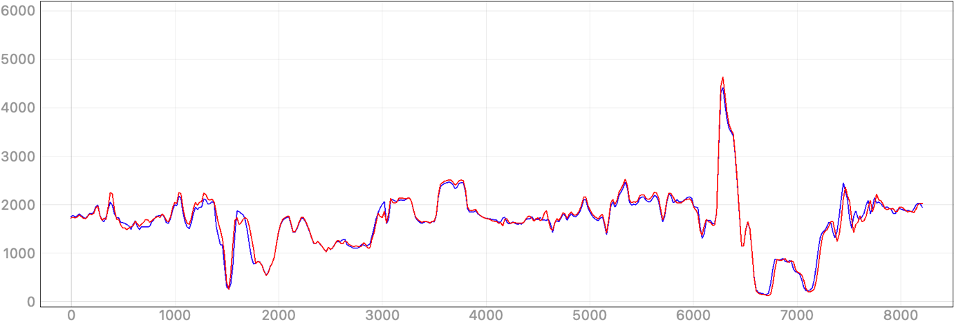
Figure A1-9: Band 11 (i.e., SWIR1 band) reflectance (with a scaling factor of 10,000) profiles for the ESA-Copernicus (in blue) and Sen2Cor version 2.5.5 (in red) Level2-A products (on 8 May 2017), Laugharne-River Tâf- River Towy transect.
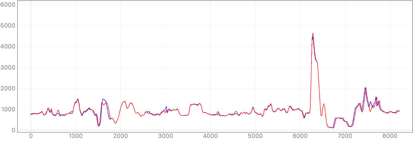
Figure A1-10: Band 12 (i.e., SWIR2 band) reflectance (with a scaling factor of 10,000) profiles for the ESA-Copernicus (in blue) and Sen2Cor version 2.5.5 (in red) Level2-A products (on 8 May 2017), Laugharne-River Tâf- River Towy transect.
Appendix 2: Eglwyswrw transect
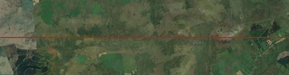
Figure A2-1: Localisation of the Eglwyswrw transect
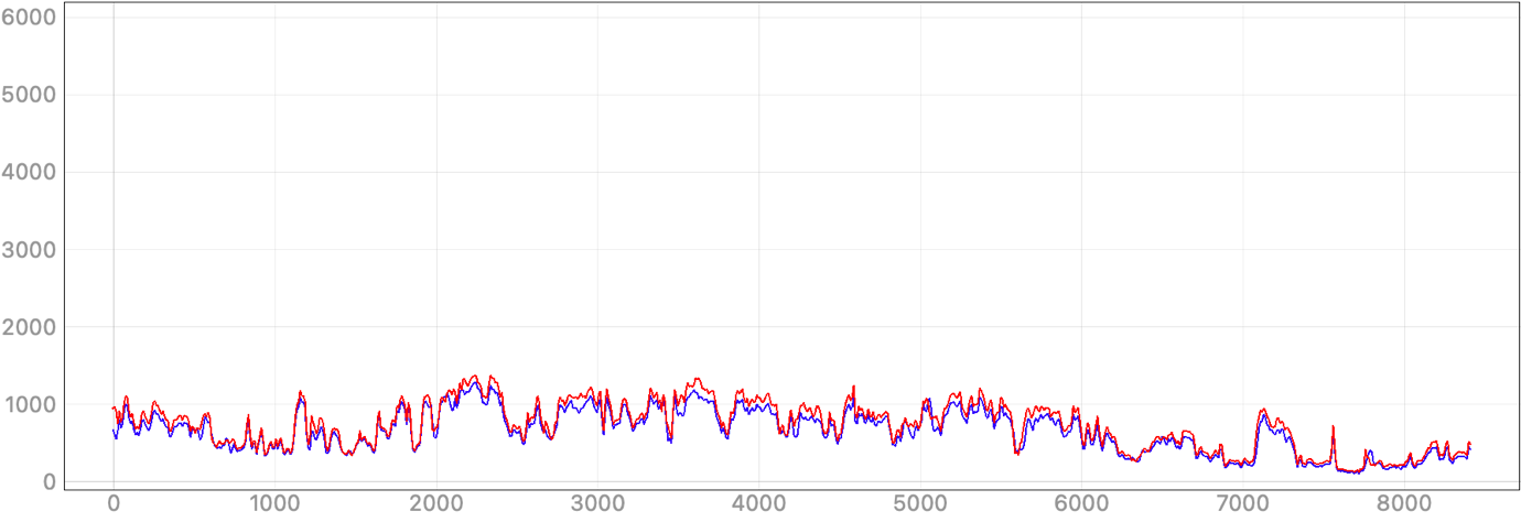
Figure A2-2: Band 2 (i.e., blue band) reflectance (with a scaling factor of 10,000) profiles for the ESA-Copernicus (in blue) and Sen2Cor version 2.5.5 (in red) Level2-A products (on 8 May 2017), Eglwyswrw transect.
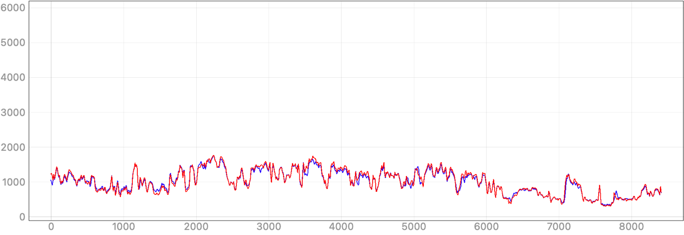
Figure A2-3: Band 3 (i.e., green band) reflectance (with a scaling factor of 10,000) profiles for the ESA-Copernicus (in blue) and Sen2Cor version 2.5.5 (in red) Level2-A products (on 8 May 2017), Eglwyswrw transect.
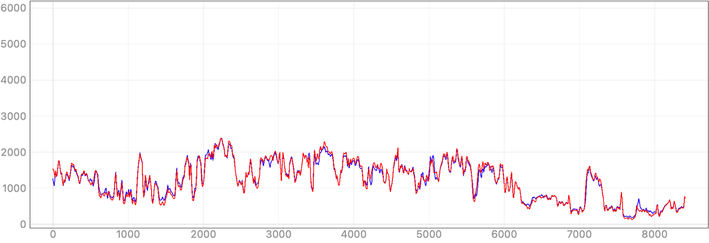 Figure A2-4: Band 4 (i.e., red band) reflectance (with a scaling factor of 10,000) profiles for the ESA-Copernicus (in blue) and Sen2Cor version 2.5.5 (in red) Level2-A products (on 8 May 2017), Eglwyswrw transect.
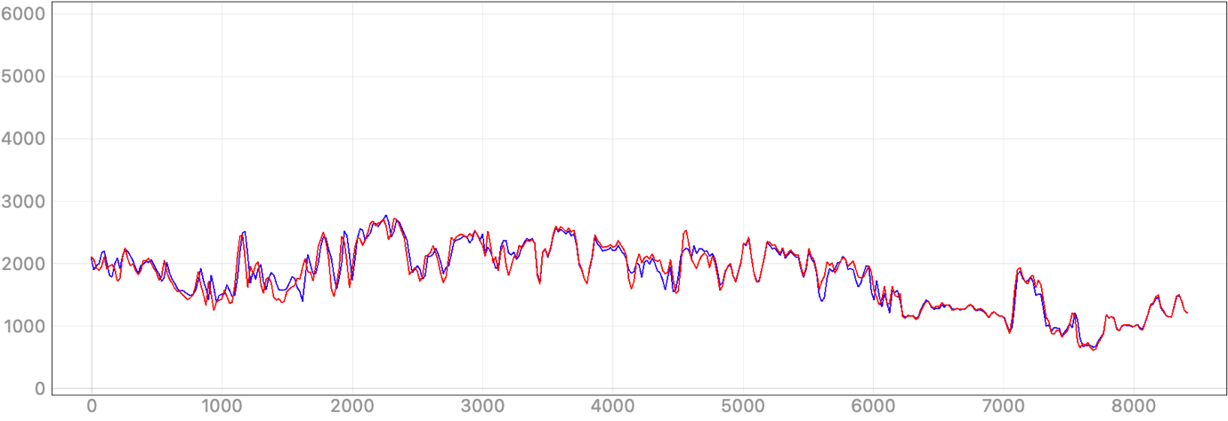
Figure A2-5: Band 5 (i.e., vegetation red edge) reflectance (with a scaling factor of 10,000) profiles for the ESA-Copernicus (in blue) and Sen2Cor version 2.5.5 (in red) Level2-A products (on 8 May 2017), Eglwyswrw transect.
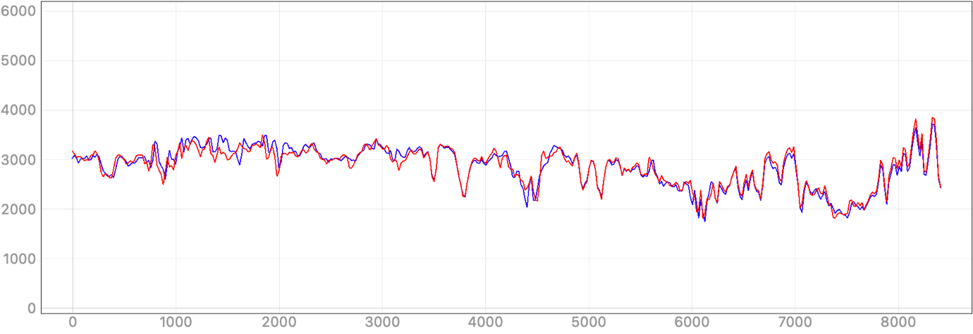
Figure A2-6: Band 6 (i.e., vegetation red edge) reflectance (with a scaling factor of 10,000) profiles for the ESA-Copernicus (in blue) and Sen2Cor version 2.5.5 (in red) Level2-A products (on 8 May 2017), Eglwyswrw transect.
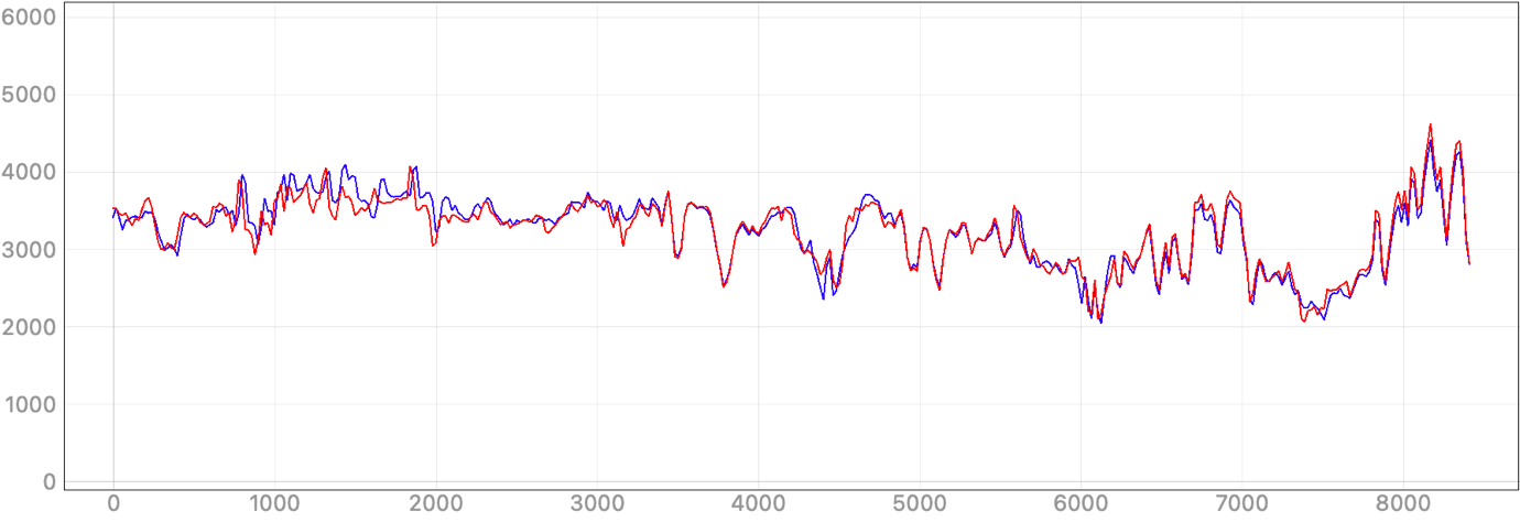
Figure A2-7: Band 7 (i.e., vegetation red edge) reflectance (with a scaling factor of 10,000) profiles for the ESA-Copernicus (in blue) and Sen2Cor version 2.5.5 (in red) Level2-A products (on 8 May 2017), Eglwyswrw transect.
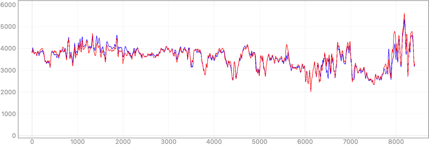
Figure A2-8: Band 8 (i.e., NIR band) reflectance (with a scaling factor of 10,000) profiles for the ESA-Copernicus (in blue) and Sen2Cor version 2.5.5 (in red) Level2-A products (on 8 May 2017), Eglwyswrw transect.
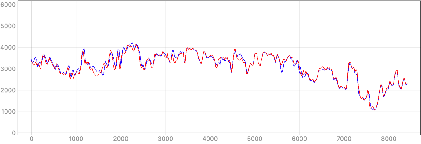
Figure A2-9: Band 11 (i.e., SWIR1 band) reflectance (with a scaling factor of 10,000) profiles for the ESA-Copernicus (in blue) and Sen2Cor version 2.5.5 (in red) Level2-A products (on 8 May 2017), Eglwyswrw transect.
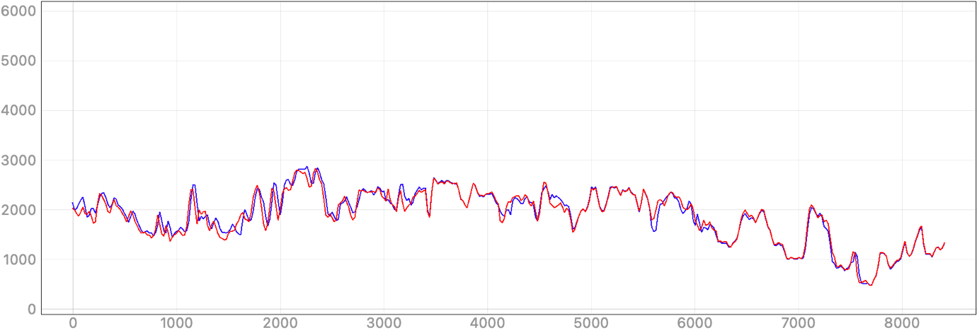
Figure A2-10: Band 12 (i.e., SWIR2 band) reflectance (with a scaling factor of 10,000) profiles for the ESA-Copernicus (in blue) and Sen2Cor version 2.5.5 (in red) Level2-A products (on 8 May 2017), Eglwyswrw transect.